Physical Address
304 North Cardinal St.
Dorchester Center, MA 02124
Physical Address
304 North Cardinal St.
Dorchester Center, MA 02124

Another stroll back in time here to talk about the way we order data and how it affects how efficiently we can store, retrieve, and analyze it. Sorting a single-dimensional list is straightforward, but real-world data is often multi-dimensional – geospatial coordinates, time-series signals, image pixels, or high-dimensional vectors.
Enter the Hilbert Curve, a 19th-century mathematical construction that provides a way to map multi-dimensional space into a one-dimensional sequence while preserving locality. What began as a mathematical curiosity is now embedded in database engines, spatial indexes, and machine learning pipelines.
This post explores the history of the Hilbert Curve, explains why it matters and presents some simple Python code to generate the curves and impress your friends.
The Hilbert urve was introduced in 1891 by David Hilbert, one of the most influential mathematicians of the late 19th and early 20th centuries.

Hilbert was exploring space-filling curves, continuous curves that pass through every point of a multi-dimensional space. At first glance, this seems impossible. How can a one-dimensional curve fully cover a two-dimensional plane? Yet Hilbert, following work by Giuseppe Peano, constructed such curves using recursive subdivisions. The more I read about Hilbert, the more I am amazed by his vision and genius.
Why does this matter? Because these curves provide a way to linearize multidimensional data while preserving locality, in lamen terms they allow points close in 2D or 3D space remain close along the curve.
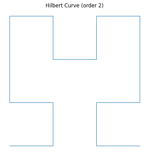
A Hilbert curve is constructed recursively:
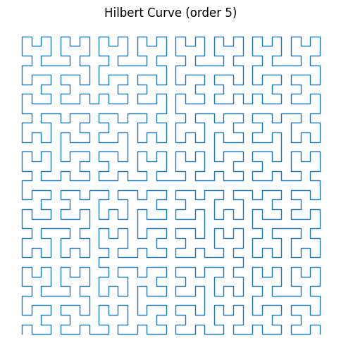
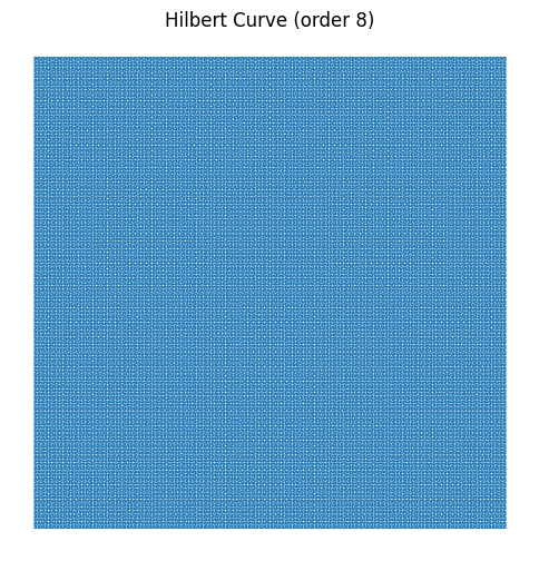
Let’s walk through a simple example to show Hilbert Curves with different orders (I’ve highlighted the row you need to change the order of the curve you generate).
import math
import matplotlib.pyplot as plt

def _rot(n, x, y, rx, ry):
    """Rotate/flip a quadrant appropriately (helper for Hilbert mapping)."""
    if ry == 0:
        if rx == 1:
            x = n - 1 - x
            y = n - 1 - y
        x, y = y, x  # swap
    return x, y

def hilbert_index_to_xy(order, d):
    """
    Convert Hilbert curve index d to (x, y) on a 2^order x 2^order grid.
    order >= 1, d in [0, 4^order - 1].
    """
    n = 1 << order  # grid size = 2^order
    x = y = 0
    t = d
    s = 1
    while s < n:
        rx = 1 & (t // 2)
        ry = 1 & (t ^ rx)
        x, y = _rot(s, x, y, rx, ry)
        x += s * rx
        y += s * ry
        t //= 4
        s <<= 1
    return x, y

def hilbert_points(order):
    """Generate points along the Hilbert curve for a given order."""
    n = 1 << order
    total = n * n
    return [hilbert_index_to_xy(order, d) for d in range(total)]

# --- Demo: plot an order-6 Hilbert curve ---
order = 3  # try 4..8
pts = hilbert_points(order)

# Scale to [0,1] for a tidy plot
n = 1 << order
xs = [x / (n - 1) for x, _ in pts]
ys = [y / (n - 1) for _, y in pts]

plt.figure(figsize=(6, 6))
plt.plot(xs, ys, linewidth=1)
plt.axis("equal")
plt.axis("off")
plt.title(f"Hilbert Curve (order {order})")
plt.show()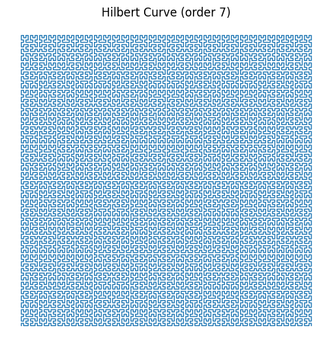


The core challenge in databases with spatial or multi-dimensional data is indexing. You want queries like:
Naïve row-by-row scans are way too slow. Traditional B-trees only order by one key. The Hilbert curve provides a space-filling curve index that reduces multidimensional search into a range scan in one dimension. Where can we see this today?
Many modern systems use Hilbert ordering as a compromise: mathematically strong locality preservation + easy mapping to integers.
Storing latitude/longitude as Hilbert indices allows fast spatial queries. For example:
Pixels in an image can be ordered along a Hilbert curve to preserve spatial locality in compression, cache-friendly storage, and texture mapping.
Columnar stores use Hilbert ordering to cluster multi-dimensional data for efficient scans. Example: clustering by (region, product, time) so that related queries touch fewer blocks.
Particle simulations and finite-element methods map 3D space to Hilbert order to improve memory locality in HPC workloads.
Vector databases and approximate nearest neighbor (ANN) search can use Hilbert ordering as a preprocessing step to cluster embeddings.
David Hilbert is famous not just for space-filling curves but for his 23 problems, presented in 1900, which defined much of 20th-century mathematics. The Hilbert Curve was an early exploration of infinity, dimensionality, and geometry. It seemed abstract at the time, but today it’s a cornerstone of practical data engineering.
This is a classic example of how pure mathematics anticipates real-world computing needs decades (sometimes a century) ahead of time.
ST_HilbertCode() for mapping geometries into Hilbert order.-- Example in PostgreSQL with PostGIS extension
SELECT ST_MakeLine(geom ORDER BY geom) AS geom FROM points;Like every solution, there are domains it does not perform as well at.
Despite this, for 2–6 dimensions (typical in geospatial, OLAP, and time-series), Hilbert is still an excellent choice.
The Hilbert Curve is a bridge between abstract 19th-century mathematics and 21st-century data systems. You don’t need to understand it at a deep mathematical level, but it’s fascinating to learn techniques introduced over a hundred years ago are critical to modern database processing. By providing a way to map multidimensional points into a one-dimensional order while preserving spatial locality, it underpins geospatial databases, OLAP stores, and even machine learning applications.
When you query for “all users within 5km of London” or when a database efficiently clusters multidimensional data, there’s a good chance Hilbert’s curve is quietly at work.
What began as a mathematical curiosity is now a practical tool of data architecture, again, a perfect reminder that today’s data problems often have roots in yesterday’s mathematics.


You must be logged in to post a comment.